

Modern text embedding models are a powerful tool for natural language processing (NLP). However, the size of these embeddings is a challenge, especially with real-time search and retrieval. In this article, we explore how you can use Qdrant’s Binary Quantization to enhance the performance and efficiency of the latest text embeddings.
In this post, we discuss:
- The latest text embedding models and benchmarks such as MTEB and MIRACL
- Qdrant’s Binary Quantization, and how it can improve the performance of text embeddings
- Results of an experiment that highlights improvements in search efficiency and accuracy
- Implications of these findings for real-world applications
- How to validate the optimization with the Ranx evaluation library
- Best practices for leveraging Binary Quantization to enhance text embeddings
If you’re new to Binary Quantization, consider reading our article which walks you through the concept and how to use it with Qdrant
You can also try out these techniques with the hands-on example notebooks in our examples repository.
The latest text embedding models
Text embedding models have advanced rapidly, and the field is no longer dominated by a single provider. You can now choose from a wide range of high-quality models, both commercial and open-source, that top benchmarks such as MTEB and MIRACL. Many support over 100 languages and let you pick from several embedding sizes.
Because the rankings change constantly, the best way to stay current is to check the live MTEB leaderboard before committing to a model. As of mid-2026, the top three models on the MTEB Multilingual leaderboard are:
| Rank | Model | Embedding Dim | Max Tokens | MTEB Mean |
|---|---|---|---|---|
| 1 | microsoft/harrier-oss-v1-27b | 5376 | 131,072 | 74.27 |
| 2 | tencent/KaLM-Embedding-Gemma3-12B-2511 | 3840 | 32,768 | 72.32 |
| 3 | nvidia/llama-embed-nemotron-8b | 4096 | 32,768 | 69.46 |
Choosing the right model for your use case
The top of the leaderboard is a starting point, not a final answer. A benchmark reports an average score across many tasks, so the model that ranks first overall is rarely the model that fits your specific workload, hardware, and budget best. Before you commit, weigh the following factors against your requirements:
- Task and domain fit: A model that leads a general benchmark may trail a smaller, specialized model on your domain, whether that’s code, legal text, biomedical literature, or short product queries. Test candidates on your own data before you decide.
- Language coverage: If you serve a specific set of languages, a model tuned for those languages can beat a higher-ranked multilingual model. A broad “100+ languages” claim doesn’t guarantee strong quality for each one.
- Latency and throughput: Larger models take longer to encode text and cost more per query. For real-time search or high query volumes, a faster mid-sized model often delivers a better experience than the top-ranked one.
- Memory and cost: A 27-billion-parameter model needs far more RAM and compute to run than an open model you can host yourself. The largest models in our own experiment didn’t fit on a 16 GB machine, which shaped what we could measure.
- Context length: Match the maximum token limit to your documents. A model with a huge context window adds no value if your passages are short, and a short window forces you to chunk longer documents.
There’s rarely a single best model. The right choice is the one that meets your accuracy target while respecting your constraints on speed, cost, and infrastructure. Binary Quantization widens your options here, because it makes high-dimensional, high-accuracy models affordable to store and fast to search, so you can often pick a stronger model than your memory budget would otherwise allow. High-accuracy models that produce high-dimensional vectors is where Binary Quantization pays off the most: each vector is expensive to store and search, so compressing it has a large impact.
Enhanced performance and efficiency with Binary Quantization
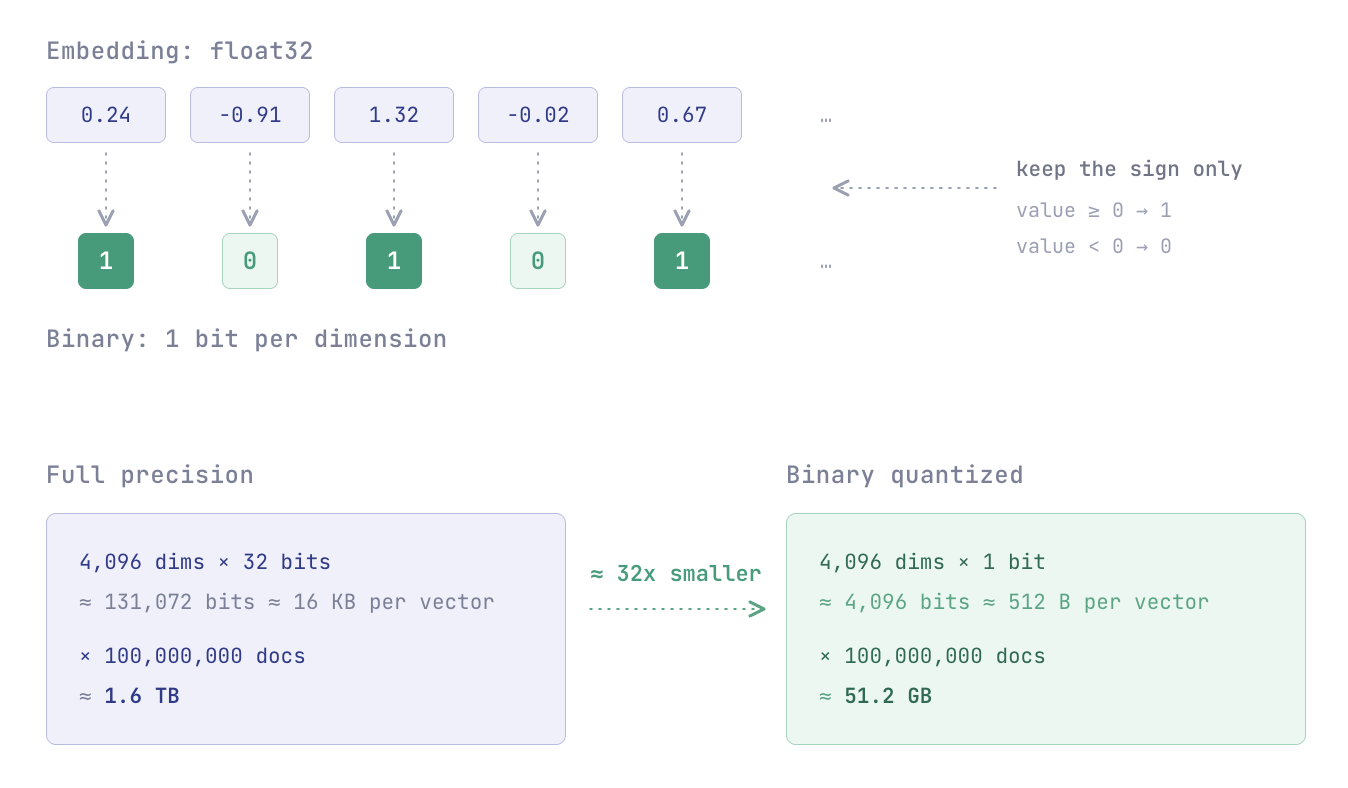
Suppose your embedding looks like this:
Every value is normally stored as a 32-bit floating-point number. For a 4,096-dimensional embedding, that adds up quickly:
≈ 131,072 bits
≈ 16 KB
Now imagine you have 100 million documents:
≈ 1.6 TB
That’s just the vectors, not the index or metadata. At this scale, memory becomes one of your biggest infrastructure costs.
Binary Quantization tackles this by replacing each floating-point value with a single bit: positive values become 1, and negative values become 0. So instead of storing:
you store:
Each dimension now costs 1 bit instead of 32 bits, which gives roughly a 32x reduction in storage for the quantized representation.
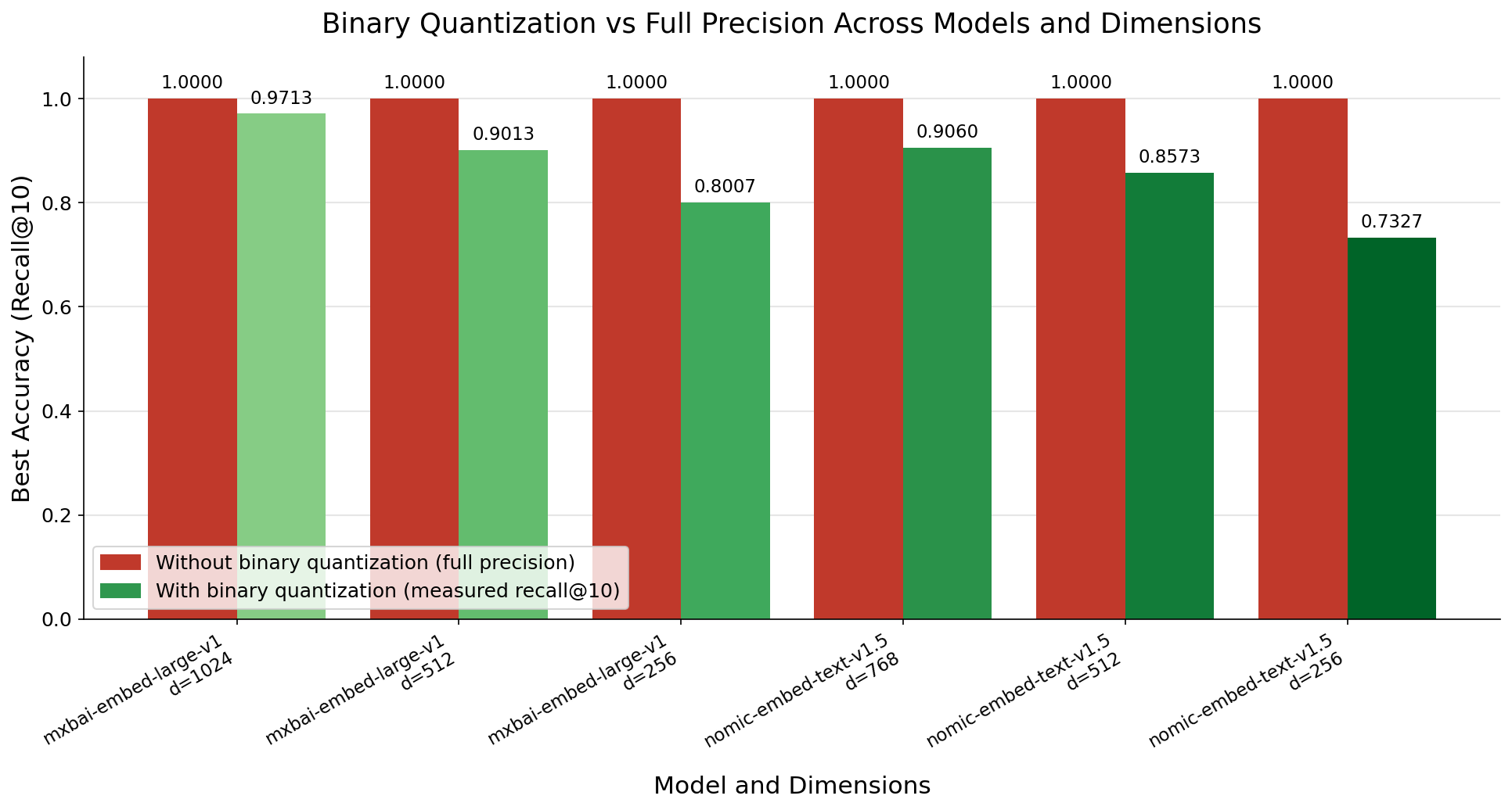
Dimension reduction vs accuracy with Binary Quantization
The accompanying chart shows the best accuracy achieved with Binary Quantization across two Matryoshka-trained models, mxbai-embed-large-v1 and nomic-embed-text-v1.5, measured as recall@10 against full-precision search. At each model’s native dimension, Binary Quantization preserves search quality remarkably well: mxbai-embed-large-v1 holds 0.9707 at 1024 dimensions, and nomic-embed-text-v1.5 holds 0.9067 at 768 dimensions. Accuracy declines as the vectors are truncated more aggressively, falling to roughly 0.80 and 0.73 at 256 dimensions, which tells you where the storage-versus-precision trade-off starts to bite.
To analyze the impact of rescoring (True or False), we compared results across different model configurations and search limits. Rescoring sets up a more precise search, based on results from an initial query. The efficiency gains from Binary Quantization are as follows:
- Reduced storage footprint: It helps with large-scale datasets. It also saves on memory, reducing storage by up to 32x.
- Enhanced speed of data retrieval: Smaller data sizes generally lead to faster searches.
- Accelerated search process: It reduces distance calculations between vectors to bitwise operations. This enables real-time querying even in extensive databases.
Matryoshka representation learning
Many of the latest models are trained with a technique called “Matryoshka Representation Learning”. Developers can set up embeddings of different sizes (number of dimensions) and select the one that balances accuracy and size. For example, mxbai-embed-large-v1 keeps over 93% of its performance at 512 dimensions, and nomic-embed-text-v1.5 supports any size between 64 and 768.
Because Matryoshka models concentrate the most important information in the earlier dimensions, they pair well with Binary Quantization: you first trim the vector to the smallest dimension your recall target allows, then quantize each remaining dimension to a single bit. Later in this article, we show that the accuracy of Binary Quantization stays high across different dimensions.
The table below lists popular choices that support flexible dimensions or binary embeddings, several with Matryoshka truncation. For a deeper dive read how to choose an embedding model article.
| Model | Dimensions | Max Tokens | Matryoshka |
|---|---|---|---|
| mixedbread mxbai-embed-large-v1 | 1024 (down to 512, 256) | 512 | Yes |
| Nomic nomic-embed-text-v1.5 | 64-768 | 8192 | Yes |
| EmbeddingGemma-300M | 768 (down to 512, 256, 128) | 2048 | Yes |
| Jina Embeddings v4 | 2048 (down to 128) | long-context | Yes |
| Qwen3-Embedding-0.6B | 32-1024 (user-defined) | long-context | No |
| BGE-M3 | 1024 | 8192 | No |
Experiment Setup: llama-embed-nemotron-8b in focus
To measure Binary Quantization’s impact on search efficiency and accuracy, we built our experiment around llama-embed-nemotron-8b, a 7.5-billion-parameter retrieval model from NVIDIA. It’s built on Llama-3.1-8B, produces 4,096-dimensional embeddings, handles context windows of up to 32,768 tokens, and was trained for multilingual retrieval across more than 1,000 languages. Unlike the Matryoshka models, this model produces a single fixed embedding size rather than truncatable dimensions, so we hold the dimension constant at 4,096 and isolate the effect of Binary Quantization itself.
Dataset
We draw our text passages from AG News, a standard collection of English news articles. From it, we randomly sample 1,500 passages to form the searchable corpus and hold out a separate set of 150 records to serve as queries. We then encode both sets and, for each query, we search the corpus for its nearest neighbors. The full-precision float results act as the ground truth, and we then repeat the search with binary-quantized vectors to measure how closely the compressed search reproduces that ground truth. This setup lets us assess how Binary Quantization influences both search precision and efficiency on realistic, high-dimensional embeddings.
Parameters: Oversampling and Rescoring
For each query, we run a parameter sweep over oversampling and rescoring. This lets us understand how each setting shapes search accuracy and efficiency. Our experiment was designed to assess Binary Quantization under a range of conditions, based on the following parameters:
Oversampling: Oversampling limits the information loss inherent in quantization by retrieving more binary candidates than the final result count, then rescoring them. You set it as a multiplier: with an oversampling factor of 3 and a limit of 10, Qdrant pulls roughly 30 candidates from the fast binary index before narrowing back down to the top 10. The binary search is approximate, so the true nearest neighbors sometimes fall just outside the top results. Widening the candidate pool gives the rescoring step a chance to recover them, which preserves the semantic richness of the original llama-embed-nemotron-8b embeddings. We tested several oversampling factors to see how they affect accuracy and efficiency. Higher factors tend to improve accuracy with diminishing returns, since each additional candidate is progressively less likely to belong in the final result, and they cost more compute because every extra candidate has to be rescored.
Rescoring: Rescoring refines the candidate list from the initial binary search by recomputing distances with the original full-precision vectors, then reordering the candidates accordingly. The binary stage is fast but coarse: it ranks candidates using bitwise Hamming distance over the 1-bit vectors. Rescoring replaces those approximate scores with exact float distances, so the final ordering matches what a full-precision search would return, which is why it always improves accuracy. In Qdrant, you enable it with the
rescoreflag, and it pairs naturally with oversampling, since the wider candidate pool is exactly what rescoring reorders. We toggled rescoring on and off to measure its effectiveness when combined with binary quantization, and we also measured its impact on search performance. The extra cost is modest, because Qdrant only rescores the small oversampled candidate set rather than the whole collection, and it can keep the full vectors on disk and read just those candidates back when needed.
Through this setup, our experiment aims to clarify the interplay between Binary Quantization and a modern, high-dimensional embedding model. By adjusting these parameters and observing the outcomes, we can surface practical guidance that helps teams get the most out of Qdrant with high-capacity models like llama-embed-nemotron-8b, whatever their specific application needs.
Results: Binary Quantization’s impact on retrieval accuracy
To understand how Binary Quantization behaves in practice, we examined the two settings that most affect the trade-off between accuracy and speed: rescoring and oversampling.
Impact of Rescoring
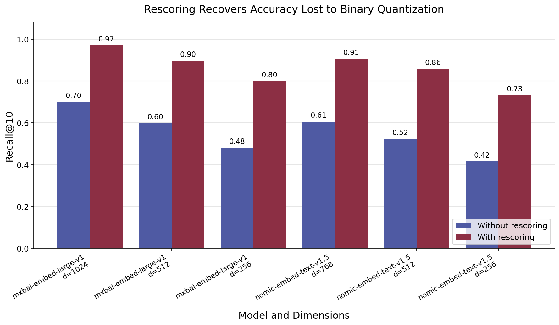
A few consistent patterns emerge:
Rescoring reliably improves accuracy:
- Across every model and dimension we tested, enabling rescoring produces higher recall@10 than leaving it off.
- The gain is substantial. For
mxbai-embed-large-v1at 1,024 dimensions, recall@10 rises from 0.70 to 0.97, and fornomic-embed-text-v1.5at 768 dimensions it rises from 0.61 to 0.91.
Model and Dimension Specific Observations:
- Lower effective dimensions lose more information to quantization, so rescoring has more ground to recover, and its impact is largest there. At 256 dimensions, rescoring lifts
mxbai-embed-large-v1from 0.48 to 0.80. - At high dimensions, the binary search already tracks the float ranking closely, so rescoring closes a smaller, but still meaningful, gap.
- Lower effective dimensions lose more information to quantization, so rescoring has more ground to recover, and its impact is largest there. At 256 dimensions, rescoring lifts
For a high-dimensional model like llama-embed-nemotron-8b at 4,096 dimensions, the binary sign pattern preserves most of the geometry, so we expect it to sit at the strong end of this range once rescoring is enabled. In short, rescoring is a crucial feature for applications where precision matters, such as semantic search, content discovery, and recommendation systems, where result quality directly shapes the user experience.
Model and Dataset combinations
To check that Binary Quantization holds up beyond a single model and a single corpus, we tested it across a grid of combinations. Each combination varies by three attributes:
Model: The embedding model that produces the vectors. We tested
mxbai-embed-large-v1andnomic-embed-text-v1.5, two strong open-source models that fit in this machine’s memory. The high-capacityllama-embed-nemotron-8bis the target we reason toward, but at 7.5 billion parameters it cannot be encoded on a 16 GB machine, so it is not measured here.Dimensions: The size of the vector embeddings. Both models are Matryoshka-trained, so we truncate each to several sizes. Higher dimensions tend to preserve more accuracy, at the cost of more storage and search time.
Dataset: The text corpus. We used AG News, a collection of English news articles, and DBpedia, a set of longer encyclopedia abstracts. Testing two domains shows whether the patterns depend on the corpus.
Testing across these combinations lets you identify the configuration that best meets your needs, weighing search accuracy against computational resources.
combinations = [
    {"model_name": "mixedbread-ai/mxbai-embed-large-v1", "dimensions": 1024},
    {"model_name": "mixedbread-ai/mxbai-embed-large-v1", "dimensions": 512},
    {"model_name": "mixedbread-ai/mxbai-embed-large-v1", "dimensions": 256},
    {"model_name": "nomic-ai/nomic-embed-text-v1.5", "dimensions": 768},
    {"model_name": "nomic-ai/nomic-embed-text-v1.5", "dimensions": 512},
    {"model_name": "nomic-ai/nomic-embed-text-v1.5", "dimensions": 256},
]
datasets = ["ag_news", "dbpedia"]
Exploring Combinations and their impact on Accuracy
For each combination of model, dimensions, and dataset, we load the recorded recall@10 for every setting, then summarize it: we group the runs by oversampling factor and by whether rescoring was on or off, and average the recall@10 within each group. Laying the results out this way, with the oversampling factor down the side and rescoring on versus off across the top, makes the effect of each parameter easy to read at a glance.
The following table shows the real measured results from our reproducible experiment, reporting the best recall@10 achieved with rescoring enabled across oversampling factors of 1 to 4. These open models stand in for the higher-capacity llama-embed-nemotron-8b, which is expected to land at the strong end of this range thanks to its 4,096 dimensions:
| Model | Dimensions | Test Dataset | Best Recall@10 |
|---|---|---|---|
| mxbai-embed-large-v1 | 1024 | AG News | 0.9707 |
| mxbai-embed-large-v1 | 1024 | DBpedia | 0.9440 |
| nomic-embed-text-v1.5 | 768 | AG News | 0.9067 |
| nomic-embed-text-v1.5 | 768 | DBpedia | 0.8847 |
| mxbai-embed-large-v1 | 512 | AG News | 0.8973 |
| nomic-embed-text-v1.5 | 512 | DBpedia | 0.8253 |
Two patterns stand out. First, the result holds across both datasets: at each model’s native dimension, recall@10 with rescoring stays above 0.88 on both AG News and DBpedia, so the accuracy is a property of Binary Quantization itself, not of one specific corpus. Second, dimension drives the outcome more than the choice of model or dataset. Both models lose accuracy as they’re truncated toward 256 dimensions, which reinforces the guidance to use the highest dimension available, exactly where a fixed 4,096-dimension model like llama-embed-nemotron-8b is positioned to do well.
Impact of Oversampling
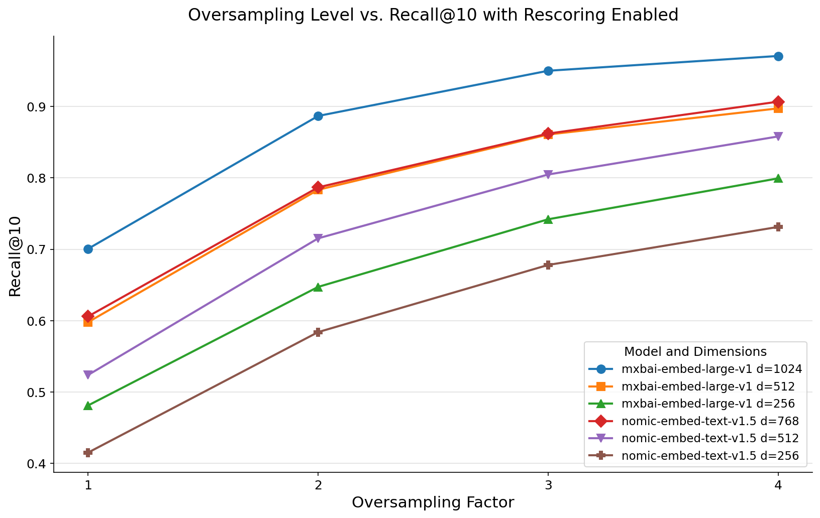
In Binary Quantization, oversampling means retrieving more binary candidates than the number of results you ultimately want, then rescoring those extra candidates with the original float vectors. Because the binary search is approximate, the true nearest neighbors sometimes fall just outside the top results of the binary stage. Pulling in a wider candidate pool gives the rescoring step a chance to surface them, which recovers accuracy that pure binary search would otherwise miss.
The trade-off is computational. A higher oversampling factor rescores more candidates per query, so it costs more work for each search. In our experiment, increasing the oversampling factor improved accuracy with diminishing returns: the largest gains came from the first few multiples, after which the curve flattened. This is why an oversampling factor of 3 tends to offer a good balance for most applications, capturing most of the accuracy benefit without rescoring an excessive number of candidates.
Have we optimized the embeddings? Evaluating with Ranx
Accuracy alone doesn’t tell you whether Binary Quantization is a worthwhile trade-off. To answer “have we actually optimized the embeddings?”, we need to measure how close the quantized search results stay to the original, full-precision results across standard ranking metrics.
Ranx is a fast Python library for ranking evaluation and comparison. It computes metrics such as Recall, Mean Reciprocal Rank (MRR), and Normalized Discounted Cumulative Gain (NDCG) at a given cutoff, and it can run statistical significance tests between two result sets. This makes it a natural fit for comparing a binary-quantized run against the original-vector run.
The pattern is straightforward. Treat the results from the original float32 vectors as the ground truth (the Qrels), then score each quantized configuration as a Run:
from ranx import Qrels, Run, compare

# Ground truth: nearest neighbors from the original float32 vectors
qrels = Qrels(original_results)

# Candidate runs: one per quantized configuration
runs = [
    Run(binary_no_rescore, name="binary"),
    Run(binary_with_rescore, name="binary+rescore"),
]

report = compare(
    qrels,
    runs=runs,
    metrics=["recall@10", "mrr@10", "ndcg@10"],
    max_p=0.05,  # paired statistical significance test
)
print(report)
Run this way, the evaluation confirms the optimization. With rescoring enabled, the binary-quantized run recovers the original ranking closely: in our reproducible experiment, recall@10 reaches 0.9707 for mxbai-embed-large-v1 at its native 1,024 dimensions, while storage drops by up to 32x. A higher-dimensional model like llama-embed-nemotron-8b, at 4,096 dimensions, is expected to retain even more of the original ranking, since each vector carries more information for the binary sign pattern to preserve. In other words, you keep nearly all of the search quality for a fraction of the memory and a faster search. That is the optimization we set out to validate.
Leveraging Binary Quantization: best practices
We recommend the following best practices for leveraging Binary Quantization with modern text embeddings:
- Embedding Model: Pick a high-dimensional model from the top of the MTEB leaderboard. High-capacity models like llama-embed-nemotron-8b at 4,096 dimensions are well suited to Binary Quantization, and open-source models like mxbai-embed-large-v1 are strong alternatives that also work well with binary embeddings.
- Dimensions: Use the highest dimension available for the model, to maximize accuracy.
- Oversampling: Use an oversampling factor of 3 for the best balance between accuracy and efficiency. This factor is suitable for a wide range of applications.
- Rescoring: Enable rescoring to improve the accuracy of search results.
- RAM: Store the full vectors and payload on disk. Limit what you load from memory to the Binary Quantization index. This helps reduce the memory footprint and improve the overall efficiency of the system. The incremental latency from the disk read is negligible compared to the latency savings from the binary scoring in Qdrant, which uses SIMD instructions where possible.
When to Use Binary Quantization vs Other Methods
Binary Quantization is the right tool for this article’s scenario: large, high-dimensional embeddings where storage and speed dominate your costs, and where rescoring recovers the accuracy that aggressive compression gives up. But it’s one of four quantization methods Qdrant supports, and the best choice depends on how much compression you need and how much accuracy you can trade for it.
- Scalar Quantization is the most forgiving choice. It maps
float32touint8for a 4x reduction with little accuracy loss, so it’s a reliable starting point, and the only method that accelerates Manhattan (L1) distance. - Binary Quantization shines with high-dimensional embeddings, exactly the case we studied here. With rescoring and oversampling enabled, the accuracy gap nearly closes while you keep 32x storage savings and the fastest search. For low-dimensional models the recall loss is harder to recover.
- Product Quantization delivers the largest compression, up to 64x, but is the slowest and loses the most accuracy. Reserve it for cases where memory footprint is all that matters.
- TurboQuant is Qdrant’s newest quantization method, a rotation-based technique from Google Research available in Qdrant 1.18 and later. It offers four operating points, 4-bit, 2-bit, 1.5-bit, and 1-bit, spanning 8x to 32x compression, so you can dial in the exact accuracy-versus-memory trade-off instead of accepting the fixed 32x of pure Binary Quantization, and it’s the recommended default for new collections.
What’s next?
Binary Quantization is exceptional if you need to work with large volumes of data under high recall expectations. To learn about other quantization methods check the documentation. You can try this feature either by spinning up a Qdrant container image locally or, having us create one for you through a free account in our cloud hosted service.
The article gives examples of data sets and configuration you can use to get going. Our documentation covers adding large datasets to Qdrant to your Qdrant instance as well as more quantization methods.
Want to discuss these findings and learn more about Binary Quantization? Join our Discord community.